Examples
This page provides worked examples for the main models supported by twowaypanel.fit(). The goal is to show typical econometric workflows: data preparation, model estimation, bias correction, inference for parameters and average partial effects (APEs), and (when applicable) MCMC convergence checks. For the full code and reproduced outputs used on this page, please refer to the accompanying Jupyter notebook:
examples.ipynb.
Data used in this page
We use two types of data in the examples below.
Binary logit / probit (empirical application): the package ships a panel dataset based on Angrist and Evans (1998), Children and their parents’ labor supply: Evidence from exogenous variation in family size (American Economic Review). The helper loader is
twowaypanel.database.angristevans98().Ordered logit / multinomial logit (simulation): we generate artificial panel data using
twowaypanel.demo.PanelGenData().For details of the artificial data generating process (DGP), please refer to the API reference for
twowaypanel.demo.PanelGenData()(see the API section of this documentation).
Throughout, the package expects:
Y: anN × Tarray (2D NumPy array is typical),X: anN × T × Karray (3D NumPy array),X_names: optional labels (list of lengthK) for readable output tables.
Import and setup
import numpy as np
import twowaypanel
Example 1: Binary logit with strictly exogenous regressors (Angrist and Evans 1998)
In this example, the dependent variable is a binary labor-force participation indicator
for married women (LFP). Regressors include indicators for the number of children
in different age bins and (log) husband income. We estimate a two-way fixed-effects
binary logit panel model.
Step 1: Load and reshape the data
The helper function twowaypanel.database.angristevans98() returns a processed
panel dataset. In practice you will typically sort by individual/time indices and
reshape into N × T (for Y) and N × T × K (for X).
data = twowaypanel.database.angristevans98()

# Typical workflow (exact variable names depend on the shipped dataset):
data = data.sort_values(["id", "year"])
N = data["id"].nunique()
T = data["year"].nunique()

# Y: LFP (N x T)
Y = data["lfp"].to_numpy().reshape(N, T)

# X: covariates (N x T x K)
X_static  = data.loc[:,['kids0_2','kids3_5','kids6_17','ln_husincome']].to_numpy().reshape(N,T,4)
X_dynamic  = data.loc[:,['lag_lfp','kids0_2','kids3_5','kids6_17','ln_husincome']].to_numpy().reshape(N,T,5)
X_static_names = ["Kids 0–2", "Kids 3–5", "Kids 6–17", "ln(hus inc)"]
X_dynamic_names = ["LFP_t-1", "Kids 0–2", "Kids 3–5", "Kids 6–17", "ln(hus inc)"]
Note
For nonlinear fixed-effects models, some individuals/time periods can be under-identified (e.g., no within-individual variation in the outcome). The package will drop such units and report how many were removed.
Step 2: Joint MLE (no bias correction)
res_mle = twowaypanel.fit(
    lfp, X_static,
    model="logit", prior=None,
    algorithm="JML",
    X_names=X_static_names
)
Output
--------------------------------------------------------------------------------
---- ESTIMATION RESULTS --------------------------------------------------------
                 LOGIT PANEL MODEL WITH TWO-WAY FIXED EFFECTS
                           WITHOUT BIAS CORRECTION
--------------------------------------------------------------------------------
Number of Individuals:   664                              Observations:     5976
Number of Time Periods:    9                            Log-likelihood: -3033.74
Algorithm: Joint MLE                              Time spent (seconds):    3.190
--------------------------------------------------------------------------------
Independent variable    Coefficient     Std. Err.   P>|z|   [95% conf. interval]
--------------------------------------------------------------------------------
            Kids 0–2   -1.17434565    0.09836036   0.000    -1.36713   -0.98156
            Kids 3–5   -0.59134501    0.08622960   0.000    -0.76035   -0.42234
           Kids 6–17   -0.01566283    0.06075953   0.797    -0.13474    0.10342
         ln(hus inc)   -0.40458145    0.09432568   0.000    -0.58945   -0.21971
--------------------------------------------------------------------------------

--------------------------------------------------------------------------------
---- AVERAGE PARTIAL EFFECTS ---------------------------------------------------
--------------------------------------------------------------------------------
Independent variable    Coefficient     Std. Err.   P>|z|   [95% conf. interval]
--------------------------------------------------------------------------------
            Kids 0–2   -0.08946279    0.03765011   0.018    -0.16326   -0.01566
            Kids 3–5   -0.04504924    0.01961088   0.022    -0.08348   -0.00662
           Kids 6–17   -0.00119321    0.00463185   0.797    -0.01027    0.00788
         ln(hus inc)   -0.03082141    0.01526161   0.044    -0.06073   -0.00091
--------------------------------------------------------------------------------
Note: Panel data contains under-identified observations;
      Dropped 797 out of 1461 individuals, and 0 out of 9 time periods.
The “Dropped … individuals” message is expected in nonlinear fixed-effects models: individuals with no within variation in outcomes contribute little/no information for identifying the slope parameters.
Example 2: Binary logit with strictly exogenous regressors + model-specific prior (MCMC) + convergence diagnostics
This example illustrates two features:
Using a model-specific bias-reducing prior (tailored for exponential-family models with strictly exogenous regressors).
Running the Metropolis–Hastings sampler (
algorithm="MCMC") and checking convergence.
beta_variance = np.array([np.sqrt(1e-1),np.sqrt(1e-2),np.sqrt(1e-2),np.sqrt(5e-5),np.sqrt(5e-7)])

res_mcmc = twowaypanel.fit(
    lfp, X_static,
    model="logit", prior="SE", algorithm="MCMC",
    X_names=X_static_names,
    beta_variance=beta_variance,fe_variance=0.1,
    mcmc_iters=150000, mcmc_burnin=50000, mcmc_skipsize=20,
    mcmc_timer=1, mcmc_sv_mle=True, mcmc_diagnosis=True
)
Output
--------------------------------------------------------------------------------
---- ESTIMATION RESULTS --------------------------------------------------------
                 LOGIT PANEL MODEL WITH TWO-WAY FIXED EFFECTS
             USING BIAS-REDUCING PRIOR FOR EXPONENTIAL FAMILY MODELS
                      WITH STRICTLY EXOGENOUS REGRESSORS
--------------------------------------------------------------------------------
Number of Individuals:   664                              Observations:     5976
Number of Time Periods:    9
Algorithm: Markov Chain Monte Carlo               Time spent (minutes): 3540.872
           150000 reptitions
--------------------------------------------------------------------------------
Independent variable    Coefficient     Std. Err.   P>|z|   [95% conf. interval]
--------------------------------------------------------------------------------
            Kids 0–2    -0.96974154    0.09139083   0.000    -1.14885   -0.79062
            Kids 3–5    -0.48227300    0.08078112   0.000    -0.64059   -0.32395
           Kids 6–17    0.001101959    0.05723464   0.985    -0.11107   0.113276
         ln(hus inc)    -0.37748241    0.08895669   0.000    -0.55182   -0.20313
--------------------------------------------------------------------------------

--------------------------------------------------------------------------------
---- AVERAGE PARTIAL EFFECTS ---------------------------------------------------
--------------------------------------------------------------------------------
Independent variable    Coefficient     Std. Err.   P>|z|   [95% conf. interval]
--------------------------------------------------------------------------------
            Kids 0–2    -0.09161824    0.03829473   0.017    -0.16667   -0.01656
            Kids 3–5    -0.04556369    0.01987691   0.022    -0.08452   -0.00660
           Kids 6–17    0.000104109    0.00487730   0.983    -0.00945   0.009663
         ln(hus inc)    -0.03566339    0.01644653   0.030    -0.06789   -0.00342
--------------------------------------------------------------------------------
Note: Panel data contains under-identified observations;
      Dropped 797 out of 1461 individuals, and 0 out of 9 time periods.

--------------------------------------------------------------------------------
---- MCMC DIAGNOSIS ------------------------------------------------------------
--------------------------------------------------------------------------------
                                       Geweke (1992) Convergence Diagnostic Test
                                             First 10% sample vs. 20 segments
                                                   of final 50% sample
Independent variable    Acceptance(%)    Average p-value       Smallest p-value
--------------------------------------------------------------------------------
            Kids 0–2    59.202592%            0.886                 0.744
            Kids 3–5    57.159571%            0.855                 0.682
           Kids 6–17    58.565585%            0.852                 0.689
         ln(hus inc)    30.478304%            0.573                 0.161
--------------------------------------------------------------------------------
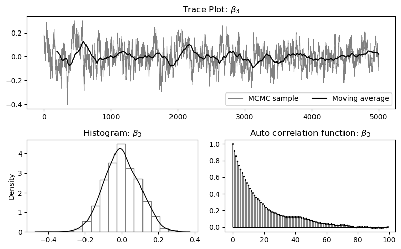
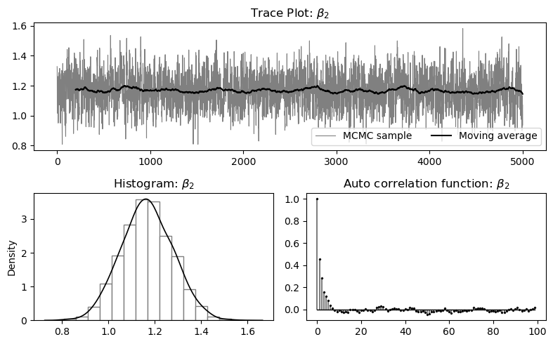
How to read the MCMC diagnostics
Acceptance rates around 20%–60% are typically reasonable for random-walk MH proposals in medium-dimensional problems (exact targets depend on tuning and blocking).
The Geweke diagnostic compares early vs late segments of the chain. Larger p-values (e.g., above 0.05) suggest no evidence against convergence (as a heuristic check).
The package also produces standard visual checks: trace plots, histograms, and autocorrelation functions (ACFs) for key common parameters.
Example diagnostic figures
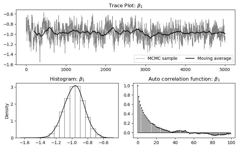
MCMC trace plot, marginal histogram, and ACF for \(\\beta_1\).

MCMC diagnostics for \(\\beta_2\).
MCMC diagnostics for \(\\beta_3\).
Example 3: Analytical bias correction (Fernández-Val and Weidner, 2016)
For binary logit/probit, you can request the analytical correction on the estimator via ac=True and prior=None.
res_fw16 = twowaypanel.fit(
    lfp, X_static,
    model="logit", prior=None, ac=True,
    algorithm="JML",
    X_names=X_static_names
)
Output
---- ESTIMATION RESULTS --------------------------------------------------------
                 LOGIT PANEL MODEL WITH TWO-WAY FIXED EFFECTS
                ANALYTICAL BIAS CORRECTION ON ESTIMATOR (FW16)
--------------------------------------------------------------------------------
Number of Individuals:   664                              Observations:     5976
Number of Time Periods:    9                            Log-likelihood: -3033.74
Algorithm: Joint MLE                              Time spent (seconds):    3.191
--------------------------------------------------------------------------------
Independent variable    Coefficient     Std. Err.   P>|z|   [95% conf. interval]
--------------------------------------------------------------------------------
            Kids 0–2    -1.02689349    0.09836036   0.000    -1.21966   -0.83411
            Kids 3–5    -0.51776197    0.08622960   0.000    -0.68676   -0.34876
           Kids 6–17    -0.01343869    0.06075953   0.825    -0.13252   0.105643
         ln(hus inc)    -0.35653581    0.09432568   0.000    -0.54140   -0.17166
--------------------------------------------------------------------------------

--------------------------------------------------------------------------------
---- AVERAGE PARTIAL EFFECTS ---------------------------------------------------
--------------------------------------------------------------------------------
Independent variable    Coefficient     Std. Err.   P>|z|   [95% conf. interval]
--------------------------------------------------------------------------------
            Kids 0–2    -0.09816115    0.04133108   0.018    -0.17916   -0.01715
            Kids 3–5    -0.04949307    0.02149604   0.021    -0.09162   -0.00736
           Kids 6–17    -0.00128461    0.00466036   0.783    -0.01041   0.007849
         ln(hus inc)    -0.03408139    0.01573954   0.030    -0.06492   -0.00323
--------------------------------------------------------------------------------
Note: Panel data contains under-identified observations;
      Dropped 797 out of 1461 individuals, and 0 out of 9 time periods.
Example 4: Dynamic probit with generic prior
This example illustrates a dynamic specification by including the lagged dependent variable among regressors.
res_dyn = twowaypanel.fit(
    lfp, X_dynamic,
    model="probit", prior="Generic", lag=1,
    algorithm="JML",
    X_names=X_dynamic_names
)
Output
--------------------------------------------------------------------------------
---- ESTIMATION RESULTS --------------------------------------------------------
                 PROBIT PANEL MODEL WITH TWO-WAY FIXED EFFECTS
                  USING BIAS-REDUCING PRIOR (GENERIC VERSION)
--------------------------------------------------------------------------------
Number of Individuals:   664                              Observations:     5976
Number of Time Periods:    9                            Log-likelihood: -3148.29
Algorithm: Joint MLE                              Time spent (seconds):    1.845
--------------------------------------------------------------------------------
Independent variable    Coefficient     Std. Err.   P>|z|   [95% conf. interval]
--------------------------------------------------------------------------------
             LFP_t-1    0.970193330    0.04268741   0.000    0.886530   1.053856
            Kids 0–2    -0.46261536    0.05690305   0.000    -0.57413   -0.35109
            Kids 3–5    -0.17731722    0.05122717   0.001    -0.27771   -0.07691
           Kids 6–17    0.036581388    0.03617607   0.312    -0.03432   0.107482
         ln(hus inc)    -0.22587568    0.05479406   0.000    -0.33326   -0.11848
--------------------------------------------------------------------------------

--------------------------------------------------------------------------------
---- AVERAGE PARTIAL EFFECTS ---------------------------------------------------
--------------------------------------------------------------------------------
Independent variable    Coefficient     Std. Err.   P>|z|   [95% conf. interval]
--------------------------------------------------------------------------------
             LFP_t-1    0.166942566    0.00717625   0.000    0.152877   0.181007
            Kids 0–2    -0.06130859    0.02691777   0.023    -0.11406   -0.00855
            Kids 3–5    -0.02349915    0.01179089   0.046    -0.04660   -0.00039
           Kids 6–17    0.004847987    0.00490677   0.323    -0.00476   0.014464
         ln(hus inc)    -0.02993441    0.01437215   0.037    -0.05810   -0.00176
--------------------------------------------------------------------------------
Note: The trimming parameter for estimating spectral expectation is 1.
Note: Panel data contains under-identified observations;
      Dropped 797 out of 1461 individuals, and 0 out of 9 time periods.
Use of lag option
The lag coefficient (
LFP_t-1) is large and precisely estimated, reflecting substantial persistence in labor-force participation.The trimming parameter
lag=1controls the truncation level for estimating spectral expectation objects entering bias correction.
Example 5: Ordered logit (simulated data)
Here we generate a dynamic ordered-logit panel with two-way fixed effects. The DGP is produced by
twowaypanel.demo.PanelGenData().
Generating artificial data
# Generate a dynamic ordered-logit panel (returns long-form arrays by default)
FEi, FEt, FE, index_i, index_t, Y, X, Ystar, alphas0, gammas0 = twowaypanel.demo.PanelGenData(
    N=45, T=15, seed=10, model="ologit", dynamic=1
)

# Reshape into N x T and N x T x K
Y = Y.reshape(45, 15)
X = X.reshape(45, 15, 2)
MLE without correction vs generic prior
res_ologit_mle = twowaypanel.fit(
    Y, X, model="ologit",
    prior=None, algorithm="JML",
    cutoff0=-2.5,      # identification normalization
)


res_ologit_generic = twowaypanel.fit(
    Y, X, model="ologit",
    prior="Generic", algorithm="JML", lag=1,
    cutoff0=-2.5,
)
--------------------------------------------------------------------------------
---- ESTIMATION RESULTS --------------------------------------------------------
               ORDERED LOGIT PANEL MODEL WITH TWO-WAY FIXED EFFECTS
                           WITHOUT BIAS CORRECTION
--------------------------------------------------------------------------------
Number of Individuals:    45                              Observations:      675
Number of Time Periods:   15                            Log-likelihood:  -685.19
Algorithm: Joint MLE                              Time spent (seconds):    0.053
--------------------------------------------------------------------------------
                        Coefficient     Std. Err.   P>|z|   [95% conf. interval]
--------------------------------------------------------------------------------
                  X1    0.441343774    0.18110680   0.015    0.086392   0.796295
                  X2    1.241542606    0.11763947   0.000    1.010980   1.472104
--------------------------------------------------------------------------------
            /cutoff2    0.466886524    0.17628462   0.008    0.121386   0.812386
            /cutoff3    2.698815569    0.22275833   0.000    2.262231   3.135399
--------------------------------------------------------------------------------

--------------------------------------------------------------------------------
---- AVERAGE PARTIAL EFFECTS ---------------------------------------------------
--------------------------------------------------------------------------------
             Pr(Y=1)    Coefficient     Std. Err.   P>|z|   [95% conf. interval]
--------------------------------------------------------------------------------
                  X1    0.030253733    0.01309578   0.021    0.004587   0.055920
                  X2    0.084568510    0.01406633   0.000    0.056999   0.112137
--------------------------------------------------------------------------------
             Pr(Y=2)    Coefficient     Std. Err.   P>|z|   [95% conf. interval]
--------------------------------------------------------------------------------
                  X1    0.048848728    0.02139962   0.022    0.006907   0.090789
                  X2    0.131727845    0.01749094   0.000    0.097447   0.166008
--------------------------------------------------------------------------------
             Pr(Y=3)    Coefficient     Std. Err.   P>|z|   [95% conf. interval]
--------------------------------------------------------------------------------
                  X1    -0.03211661    0.01563286   0.040    -0.06275   -0.00147
                  X2    -0.08122116    0.01867050   0.000    -0.11781   -0.04462
--------------------------------------------------------------------------------
             Pr(Y=4)    Coefficient     Std. Err.   P>|z|   [95% conf. interval]
--------------------------------------------------------------------------------
                  X1    -0.04698584    0.01937041   0.015    -0.08494   -0.00902
                  X2    -0.13507518    0.01714204   0.000    -0.16867   -0.10147
--------------------------------------------------------------------------------


--------------------------------------------------------------------------------
---- ESTIMATION RESULTS --------------------------------------------------------
               ORDERED LOGIT PANEL MODEL WITH TWO-WAY FIXED EFFECTS
                  USING BIAS-REDUCING PRIOR (GENERIC VERSION)
--------------------------------------------------------------------------------
Number of Individuals:    45                              Observations:      675
Number of Time Periods:   15                            Log-likelihood:  -711.48
Algorithm: Joint MLE                              Time spent (seconds):    0.080
--------------------------------------------------------------------------------
                        Coefficient     Std. Err.   P>|z|   [95% conf. interval]
--------------------------------------------------------------------------------
                  X1    0.571509060    0.17854978   0.001    0.221569   0.921448
                  X2    1.169471961    0.11501164   0.000    0.944060   1.394883
--------------------------------------------------------------------------------
            /cutoff2    0.309800227    0.16596220   0.062    -0.01546   0.635069
            /cutoff3    2.427988601    0.20935639   0.000    2.017671   2.838306
--------------------------------------------------------------------------------

--------------------------------------------------------------------------------
---- AVERAGE PARTIAL EFFECTS ---------------------------------------------------
--------------------------------------------------------------------------------
             Pr(Y=1)    Coefficient     Std. Err.   P>|z|   [95% conf. interval]
--------------------------------------------------------------------------------
                  X1    0.041244510    0.01443204   0.004    0.012959   0.069529
                  X2    0.083908563    0.01388271   0.000    0.056699   0.111117
--------------------------------------------------------------------------------
             Pr(Y=2)    Coefficient     Std. Err.   P>|z|   [95% conf. interval]
--------------------------------------------------------------------------------
                  X1    0.068221113    0.02150758   0.002    0.026068   0.110373
                  X2    0.131137738    0.01657559   0.000    0.098651   0.163624
--------------------------------------------------------------------------------
             Pr(Y=3)    Coefficient     Std. Err.   P>|z|   [95% conf. interval]
--------------------------------------------------------------------------------
                  X1    -0.04623204    0.01652339   0.005    -0.07861   -0.01384
                  X2    -0.08136355    0.01729637   0.000    -0.11526   -0.04746
--------------------------------------------------------------------------------
             Pr(Y=4)    Coefficient     Std. Err.   P>|z|   [95% conf. interval]
--------------------------------------------------------------------------------
                  X1    -0.06323357    0.02011343   0.002    -0.10265   -0.02381
                  X2    -0.13368274    0.01678849   0.000    -0.16658   -0.10077
--------------------------------------------------------------------------------
Note: The trimming parameter for estimating spectral expectation is 1.
MCMC estimation (generic prior) and convergence checks
res_ologit_mcmc = twowaypanel.fit(
    Y, X, model="ologit",
    prior="Generic", algorithm="MCMC", lag=1,
    cutoff0=-2.5,
    mcmc_iters=120000, mcmc_burnin=20000, mcmc_skipsize=20, mcmc_diagnosis=True
)
--------------------------------------------------------------------------------
---- ESTIMATION RESULTS --------------------------------------------------------
               ORDERED LOGIT PANEL MODEL WITH TWO-WAY FIXED EFFECTS
                  USING BIAS-REDUCING PRIOR (GENERIC VERSION)
--------------------------------------------------------------------------------
Number of Individuals:    45                              Observations:      225
Number of Time Periods:   15
Algorithm: Markov Chain Monte Carlo               Time spent (minutes):  177.691
           120000 reptitions
--------------------------------------------------------------------------------
                        Coefficient     Std. Err.   P>|z|   [95% conf. interval]
--------------------------------------------------------------------------------
                  X1    0.568049498    0.17823331   0.001    0.218730   0.917368
                  X2    1.167454158    0.11479293   0.000    0.942471   1.392436
--------------------------------------------------------------------------------
            /cutoff1    0.292924966    0.16484033   0.076    -0.03014   0.615995
            /cutoff2    2.400585164    0.20798825   0.000    1.992948   2.808221
--------------------------------------------------------------------------------

--------------------------------------------------------------------------------
---- AVERAGE PARTIAL EFFECTS ---------------------------------------------------
--------------------------------------------------------------------------------
             Pr(Y=0)    Coefficient     Std. Err.   P>|z|   [95% conf. interval]
--------------------------------------------------------------------------------
                  X1    0.041390922    0.01451946   0.004    0.012934   0.069847
                  X2    0.084540492    0.01391589   0.000    0.057266   0.111814
--------------------------------------------------------------------------------
             Pr(Y=1)    Coefficient     Std. Err.   P>|z|   [95% conf. interval]
--------------------------------------------------------------------------------
                  X1    0.067626969    0.02139310   0.002    0.025698   0.109555
                  X2    0.130605235    0.01649740   0.000    0.098271   0.162938
--------------------------------------------------------------------------------
             Pr(Y=2)    Coefficient     Std. Err.   P>|z|   [95% conf. interval]
--------------------------------------------------------------------------------
                  X1    -0.04584389    0.01643358   0.005    -0.07805   -0.01363
                  X2    -0.08104455    0.01721884   0.000    -0.11479   -0.04729
--------------------------------------------------------------------------------
             Pr(Y=3)    Coefficient     Std. Err.   P>|z|   [95% conf. interval]
--------------------------------------------------------------------------------
                  X1    -0.06317400    0.02016498   0.002    -0.10269   -0.02365
                  X2    -0.13410117    0.01678597   0.000    -0.16699   -0.10120
--------------------------------------------------------------------------------
Note: The trimming parameter for estimating spectral expectation is 1.

--------------------------------------------------------------------------------
---- MCMC DIAGNOSIS ------------------------------------------------------------
--------------------------------------------------------------------------------
                                       Geweke (1992) Convergence Diagnostic Test
                                             First 10% sample vs. 20 segments
                                                   of final 50% sample
Independent variable    Acceptance(%)    Average p-value       Smallest p-value
--------------------------------------------------------------------------------
                  X1    42.594425%            0.914                 0.799
                  X2    41.867418%            0.951                 0.882
            /cutoff1    36.887368%            0.942                 0.781
            /cutoff2    59.267592%            0.938                 0.770
--------------------------------------------------------------------------------
The MCMC run reports acceptance rates and Geweke diagnostics (and also produces trace/hist/ACF plots):

Diagnostics for \(\\beta_1\) in the ordered-logit example.
Diagnostics for \(\\beta_2\) in the ordered-logit example.
Example 6: Multinomial logit (simulated data)
We generate a dynamic multinomial-logit panel and compare uncorrected JML with a model-specific prior
tailored for dynamic multinomial logit (prior="PML").
_, _, _, _, _, Y, X, _, _, _ = twowaypanel.demo.PanelGenData(
    N=45, T=15, seed=10, model="mlogit", dynamic=1
)
Y = Y.reshape(45, 15)
X = X.reshape(45, 15, 2)

# Uncorrected JML
res_mlogit_mle = twowaypanel.fit(
    Y, X, model="mlogit",
    prior=None, algorithm="JML"
)

# Bias-reducing prior for dynamic multinomial logit (trimming parameter lag=1 here)
res_mlogit_dml = twowaypanel.fit(
    Y, X,
    model="mlogit", prior="PML", lag=1,
    algorithm="JML"
)
Output
--------------------------------------------------------------------------------
---- ESTIMATION RESULTS --------------------------------------------------------
             MULTINOMIAL LOGIT PANEL MODEL WITH TWO-WAY FIXED EFFECTS
                           WITHOUT BIAS CORRECTION
--------------------------------------------------------------------------------
Number of Individuals:    44                              Observations:      660
Number of Time Periods:   15                            Log-likelihood:  -590.37
Algorithm: Joint MLE                              Time spent (seconds):    0.810
--------------------------------------------------------------------------------
Independent variable    Coefficient     Std. Err.   P>|z|   [95% conf. interval]
--------------------------------------------------------------------------------
  Y = 2
                  X1    -0.02201089    0.25903835   0.932    -0.52970   0.485678
                  X2    1.006845054    0.17222417   0.000    0.669302   1.344387
  Y = 3
                  X1    0.797433329    0.26237748   0.002    0.283199   1.311666
                  X2    1.286031037    0.17948933   0.000    0.934249   1.637812
--------------------------------------------------------------------------------

--------------------------------------------------------------------------------
---- AVERAGE PARTIAL EFFECTS ---------------------------------------------------
--------------------------------------------------------------------------------
Independent variable    Coefficient     Std. Err.   P>|z|   [95% conf. interval]
--------------------------------------------------------------------------------
  Y = 2
                  X1    0.026330907    0.01542943   0.088    -0.00390   0.056571
                  X2    0.043227913    0.02556975   0.091    -0.00688   0.093342
  Y = 3
                  X1    0.028183105    0.01622722   0.082    -0.00362   0.059986
                  X2    0.120234102    0.02433605   0.000    0.072537   0.167930
--------------------------------------------------------------------------------
Note: Panel data contains under-identified observations;
      Dropped 1 out of 45 individuals, and 0 out of 15 time periods.


--------------------------------------------------------------------------------
---- ESTIMATION RESULTS --------------------------------------------------------
             MULTINOMIAL LOGIT PANEL MODEL WITH TWO-WAY FIXED EFFECTS
             USING BIAS-REDUCING PRIOR FOR EXPONENTIAL FAMILY MODELS
                         WITH PREDETERMINED REGRESSORS
--------------------------------------------------------------------------------
Number of Individuals:    44                              Observations:      660
Number of Time Periods:   15                            Log-likelihood:  -520.18
Algorithm: Joint MLE                              Time spent (seconds):    4.762
--------------------------------------------------------------------------------
Independent variable    Coefficient     Std. Err.   P>|z|   [95% conf. interval]
--------------------------------------------------------------------------------
  Y = 2
                  X1    0.284336843    0.25121981   0.258    -0.20802   0.776702
                  X2    0.926801399    0.16670645   0.000    0.600073   1.253529
  Y = 3
                  X1    0.752554189    0.25684368   0.003    0.249166   1.255942
                  X2    1.190567767    0.17313990   0.000    0.851230   1.529904
--------------------------------------------------------------------------------

--------------------------------------------------------------------------------
---- AVERAGE PARTIAL EFFECTS ---------------------------------------------------
--------------------------------------------------------------------------------
Independent variable    Coefficient     Std. Err.   P>|z|   [95% conf. interval]
--------------------------------------------------------------------------------
  Y = 2
                  X1    0.038674882    0.01617262   0.017    0.006978   0.070371
                  X2    0.041445205    0.02556205   0.105    -0.00865   0.091544
  Y = 3
                  X1    0.040827271    0.01709489   0.017    0.007322   0.074331
                  X2    0.124371599    0.02436747   0.000    0.076613   0.172129
--------------------------------------------------------------------------------
Note: The trimming parameter for estimating spectral expectation is 1.
Note: Panel data contains under-identified observations;
      Dropped 1 out of 45 individuals, and 0 out of 15 time periods.
The PML prior changes both point estimates and the fitted objective, reflecting the role of likelihood-based bias correction in finite samples.
The note about trimming parameter explains how the package approximates spectral expectations entering the correction terms in the dynamic settings with predetermined regressors.
References
Angrist, J. D., and Evans, W. N. (1998). “Children and their parents’ labor supply: Evidence from exogenous variation in family size.” American Economic Review.
Fernández-Val, I., and Weidner, M. (2016). “Individual and time effects in nonlinear panel models with large n, t.” Journal of Econometrics, 192(1), 291–312.